Unit 2 Kinetics
2.3 Integrated Rate Law
OpenStax
Section Learning Objectives
- Perform integrated rate law calculations for first-order reactions.
- Define half-life for first-order reactions and carry out related calculations.
✓ SECTION 2.3 CHECKLIST
| Learning Activity | Graded? | Estimated Time |
|---|---|---|
| Make notes about this section’s reading portion. | No | 90 min |
| Optional Resource: Watch a video explanation of integrated rate laws. | No | 2 min |
| Work on the self-check question. | No | 15 min |
| Work on practice exercises. | No | 90 min |
📖 READING PORTION
The differential rate laws discussed thus far relate the overall reaction rate and the concentrations of reactants. We can also determine a second form of rate law that relates the concentrations of reactants and time. These are called integrated rate laws. We can use an integrated rate law to determine the amount of reactant or product present after a period of time or to estimate the time required for a reaction to proceed to a certain extent. For example, an integrated rate law is used to determine the length of time a radioactive material must be stored for its radioactivity to decay to a safe level. Integrated rate laws are derived using calculus. Just as with differential rate laws, there are integrated rate laws for various orders of reactions. In CHEM 1523 , we will focus on solving problems using the first-order integrated rate law.
First-Order Integrated Rate Law
Using calculus to integrate the rate law (rate = k[A]) for a first-order reaction, A ⟶ products, results in an equation describing how the reactant concentration varies with time
Equation 1
[latex]\ln \frac{[\text{A}]}{[\text{A}]_0} = −kt[/latex]
- [latex][\text{A}][/latex], concentration of reactant A at time t
- [latex][\text{A}]_0[/latex], initial concentration of A
- [latex]k[/latex], first-order rate constant (units of inverse time)
- [latex]t[/latex], time (units of time)
Even though the equation has the concentration of A, the amount of A does not necessarily need to be a concentration. Using the mass, moles, etc. of A in the equation also works well as long as the units of A, whether concentration, mass, moles, etc., are consistent with units of the rate constant k.
For mathematical convenience, this equation may be rearranged as
Equation 2
[latex]\ln[\text{A}] = −kt + \ln [\text{A}]_0[/latex]
- [latex][\text{A}][/latex], concentration of reactant A at time t
- [latex][\text{A}]_0[/latex], initial concentration of A
- [latex]k[/latex], first-order rate constant (units of inverse time)
- [latex]t[/latex], time (units of time)
Even though the equation has the concentration of A, the amount of A does not necessarily need to be a concentration. Using the mass, moles, etc. of A in the equation also works well as long as the units of A, whether concentration, mass, moles, etc., are consistent with units of the rate constant k.
The first-order integrated rate law is also applicable for pseudo first-order reactions. For example, a reaction of the form
A + B ⟶ products
that is known to be first-order in A may be approximated as first-order overall if B is in excess. Excess B means that the concentration of B stays relatively constant, and the overall rate of the reaction will depend more on A than on B.
Example 1
The Integrated Rate Law for a First-Order Reaction
The rate constant for the first-order decomposition of cyclobutane, C4H8 at 500°C is 9.2 × 10⁻³ s−1.
C4H8 ⟶ 2 C2H4
How long will it take for 80.0% of a 1.00 M sample of C4H8 to decompose?
SOLUTION
The initial concentration of C4H8 is 1.00 M, [C4H8]0 = 1.00 M. At time t, 80.0% of C4H8 has decomposed meaning that 20.0% of C4H8 is left, [C4H8] = 0.200 M. Rearranging the rate law to isolate t and substituting the provided quantities yields
ln[C4H8] = −kt + ln[C4H8]0
ln(0.200) = −(9.2×10⁻³ s−1)t + ln(1.00)
t = 1.7 × 10² s
Graphical Approach to the Integrated Rate Law
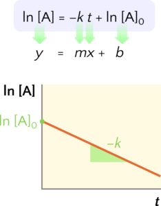
Note that if a set of rate data is plotted as ln[A] versus t but does not result in a straight line, the reaction is not first-order in A.
Example 2
Determination of Reaction Order by Graphing
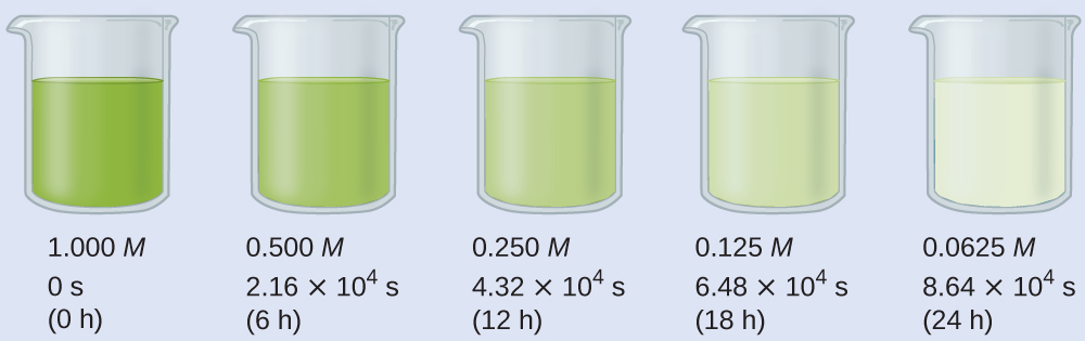
Show that the data below can be represented by a first-order rate law by graphing ln[H2O2] versus time. Determine the rate constant for the rate of decomposition of H2O2 from this data.
H2O2(aq) ⟶ H2O(l) + ½ O2(g)
| Trial | Time (h) | [H2O2] (M) | ln[H2O2] |
|---|---|---|---|
| 1 | 0 | 1.000 | 0.0 |
| 2 | 6.00 | 0.500 | −0.693 |
| 3 | 12.00 | 0.250 | −1.386 |
| 4 | 18.00 | 0.125 | −2.079 |
| 5 | 24.00 | 0.0625 | −2.772 |
SOLUTION
![A graph is shown with the label “Time ( h )” on the x-axis and “l n [ H subscript 2 O subscript 2 ]” on the y-axis. The x-axis shows markings at 6, 12, 18, and 24 hours. The vertical axis shows markings at negative 3, negative 2, negative 1, and 0. A decreasing linear trend line is drawn through five points represented at the coordinates (0, 0), (6, negative 0.693), (12, negative 1.386), (18, negative 2.079), and (24, negative 2.772).](http://principlesofchemistryopencourse.pressbooks.tru.ca/wp-content/uploads/sites/127/2022/10/CNX_Chem_12_04_FrstOKin.jpg)
The data above is plotted in Figure 2. The plot of ln[H2O2] versus time is linear, thus we have verified that the reaction may be described by a first-order rate law.
The rate constant for a first-order reaction is equal to the negative of the slope of the plot of ln[H2O2] versus time where:
In order to determine the slope of the line, we need two values of ln[H2O2] at different values of t (one near each end of the line is preferable). For example, the value of ln[H2O2] when t is 6.00 h is −0.693; the value when t = 12.00 h is −1.386:
The Half-Life of a Reaction
Equation 3
[latex]t_{1/2} = \frac{0.693}{k}[/latex]
- [latex]t_{1/2}[/latex], half-life (units of time)
- [latex]k[/latex], first-order rate constant (units of inverse time)
Example 3
Calculation of a First-Order Rate Constant using Half-Life
Calculate the rate constant for the first-order decomposition of hydrogen peroxide in water at 40°C, using the data given in Figure 3.
SOLUTION
The half-life for the decomposition of H2O2 is 2.16 × 10⁴ s:
Optional Resource
Watch a video explanation of integrated rate laws.
Video 1 Integrated Rate Laws. For CHEM 1523, we are only interested in the first-order integrated rate law (5:38-6:42).
Consider the first-order reaction
N2O5 (in CCl4) → 2 NO2(g) + ½ O2(g)
with rate constant 5.71 × 10⁻⁴ s−1. How much N2O5 is left after 600 s if the initial concentration is 0.91 M?
Click to see answer
Use the integrated rate law,
[latex]\begin{align*} \ln[\text{N}_2\text{O}_5]&=-kt+\ln[\text{N}_2\text{O}_5]_0 \\ &=-(5.71\times10^{-4}\text{ s}^{-1})(600 \text{ s})+\ln(0.91\text{ M}) \\ &=-0.44 \end{align*}[/latex]
This answer is the natural logarithm of the concentration we want. In order to isolate the concentration from the logarithm, exponentiate the logarithm.
[latex]\begin{align*} [\text{N}_2\text{O}_5]&=e^{\ln[\text{N}_2\text{O}_5]} \\ &=e^{-0.44} \\ &=\boxed{0.65\text{ M}} \end{align*}[/latex]
